Machine learning models depend on large troves of data to develop and improve their inference / prediction capabilities. These models generalize their abilities, but inevitably some of their training data is encoded or memorized within their trained parameters. This post explores a method of quantifying model memorization, factors that make models more prone to memorization, and provides some mitigations against memorization.
📌 TL;DR
- ML models tend to memorize samples from their training data, this poses a privacy risk to members whose data was part of the training dataset
- Membership Inference Attacks (MIA) are assessments which may be used to quantify model memorization, these attacks can be performed either with full access to the model or with only access to the model’s predictions
| ML models learn from training data, with the goal of generalizing what they learn to new (unseen) samples. | Despite this goal,
|
| Characteristics of the model and data affect model memorization | In general
|
| A method of assessing model privacy is the Membership Inference Attack (MIA) | / MIA / seeks to predict whether a given sample was or was not part of a model’s training dataset MIA is fundamentally a classification task (sample was in, or sample was not in the training dataset)
|
Why ML privacy matters (…and a bit of writer’s block)
I found starting this post challenging… the concern this post touches on is so foundational and broad that I found this all difficult to put into words (which is funny given my verbosity otherwise…) so I turned to an AI collaborator to help start things off: Bard.
I punted a few questions Bard’s way, and iterated on the core concepts a bit before Bard helped me write this:
" Machine learning is a rapidly evolving field with the potential to revolutionize many aspects of our lives. It is already being used in a wide range of applications: from healthcare to finance to transportation. As machine learning continues to evolve, it is likely to become even more pervasive in our lives. These ML models are often trained on large datasets of data, which can include sensitive information.
As a result, the importance of machine learning is not just limited to its potential to improve our lives. It also has the potential to impact our privacy in significant ways. "
Privacy & Machine Learning
Machine learning algorithms have become ubiquitous across products we use everyday, these algorithms attempt to generalize while necessarily being trained on a subset of all possible examples.
ML Basics & Intuition
This post is by no means an introduction to ML, there are much more skilled teachers that deliver the content in many forms of media - in particular I have enjoyed 3Blue1Brown’s series on YouTube. Some (simplified) basics for this post will do:
Generalizability
Consider a classification task: an algorithm that is trained to output one of two labels (cat or dog) using images of dogs and cats as input. If this model is trained on all sorts of cats but only large dog breeds, then we can expect it to do well on images of all sorts of cats and only large breed dogs. Even without training, this model has pretty good odds of making the correct call, a 50/50 chance of making the correct prediction without having any trained ability to differentiate dogs and cats.
Let’s say that after multiple epochs of training this same model is then tasked with classifying an image of a small breed dog that it has never seen: it may predict Dog with low confidence or worse… predict Cat.
This intuitive example reveals a little bit about how machines are capable of learning: the model attempts to “remember” a mapping from the inputs it has seen in the training data to the outputs, or the correct labels. In doing so, the model is able to map what it has seen during training to the output classes available (dog, cat). When presented with a new variant of a class it has seen then this mapping may not serve the model well.
Overfitting
Continuing this classification task example, the model is trained by:
- Being shown a picture as input (dog, cat)
- Calculating the output prediction, by cascading neuron activations throughout it’s layers
- Comparing it’s prediction against the true value, calculating it’s error
- Using back propagation alchemy to tune it’s model weights and biases to better predict that specific example
Rinse, repeat for all samples, repeat that over multiple epochs of training.
By following this procedure our classification model develops from an interconnected network of random parameters to a set of tuned parameters for its task. In general, many arbitrary ML algorithms follow this pattern: a simple regression algorithm begins with a series of random parameters and a deep neural network begins with random weights for each of its neurons and random biases for each of its connections. The process of training the model slowly tunes the trainable parameters of the model to fit its task based on the training examples that are used.
Coming back to the training process… Let’s imagine this cycle runs indefinitely - repeatedly the model is exposed to those images of all sorts of cats and only large dogs. The same pictures of all sorts of cats, and only large breed dogs. Again. And again. And again.
We can expect that as this cycle approaches the end of time said model would get really good at identifying cats and large breed dogs. That is, the model would get very skilled at predicting THOSE all sorts of cats and THOSE large breed dogs it had seen in its training data (over and over and over and…)
After each cycle of calculating losses and back propagating them through its parameters this model will overfit to the training data. In other words, the process will optimize the model’s trainable parameters to be very accurate for predicting data in it’s training dataset but will plateau or even develop this heightened accuracy at the expense of its ability to predict data outside of it’s training dataset.
What this tells us about how machines learn
Somewhere inside a trained model, within its weights and biases, this machine must retain some imprint or memory of the data it’s seen during its training. In general, models tend to perform better on samples from its training dataset, and if a model is overfit then this characteristic becomes exaggerated. The hope is that this model would generalize beyond the samples it had seen during training to new samples observed in the wild, but nonetheless its capabilities are learned during the training process.
This exploration of a model’s training and memory has profound implications for models trained on sensitive data, and especially in cases where even being a member of the training dataset reveals some sensitive characteristics about an individual.
Let’s consider a more complicated model, a classification algorithm that predicts between a finite set of theparies for a cancer patient given some data points about the patient. If an attacker has access to an individual’s data and is able to deduce the patient’s participation in the training dataset then de facto the attacker has learned that this individual has cancer and the patient’s health privacy is violated.
For such an attack, the attacker wouldn’t need access to a model’s parameters, instead the attacker would only need to have access to the model’s predictions. This is the privacy vulnerability of a model that a Membership Inference Attack exploits.
Measuring Privacy of ML Models: MIA
Membership Inference Attacks (MIA) were introduced by Shokri et al. 1 in 2017, and much of the research since its introduction has focused on improving the attack’s efficiency or proposing alternative methods to measure the same memorization tendencies of a model but the essence of the assessment remains the same: given a model and a datapoint, predict whether that datapoint was part of the model’s training dataset.
Let’s explore two MIA approaches:
1 - Membership Inference: Shadow Model Approach
Earlier, our hypothetical model classified an image as being a member of one of two possible classes: Cat or Dog.
Now we are posed with a question that also has a binary outcome: this datapoint was in or this datapoint was not in the training dataset used to train the target model. This classification task is well suited for another ML model that we will use as the attacker model.
This first MIA approach trains an attacker classification model to predict one of two possible outcomes (was in, was not in) for each class (in our example: cat, dog). This procedure is more involved, requiring more computation than the alternative because this method requires training multiple shadow ML models whose characteristics are similar to the target model we are attacking. This method also requires access to a known dataset that is similar to the target model’s training dataset, alternatively this known dataset may be generated from the target model. The shadow model approach at a high level involves two activities:
Training a set of shadow models that mirror the behavior of the target model
- These shadow models use known samples as part of their training data
- We reserve some data beyond the training data to use as validation data
Training an attacker classification model on the label (was in, was not in) and the outputs of the shadow models with the task of predicting whether a given datapoint represents a sample that was in that shadow model’s training dataset
- Since the training data for the shadow models are known, we can use these samples and the shadow models’ predictions to train our classification model to recognize model outputs on training samples
- Samples from the training data fed through the shadow models are labeled as being a member, whereas samples from the validation dataset fed through the shadow models are labeled as being nonmember. These labels are the ground truth used for the attacker models prediction error and back propagation
In Shokri et al. 1 demonstrated successful attacks using this approach with multiple shadow models. Random sampling at the onset of each shadow model’s training added entropy to the distribution of known data points into either of the training and test datasets. Later, Salem et al 2 demonstrated success using a single shadow model.
This MIA approach is often referred to as closed-system, closed-box, or black box MIA because direct access to the model’s parameters is not needed; instead only the target model’s output is needed (classification predictions, predictions confidence).
Returning to our Cat-Dog example:
Let us assume we have a set of known cat and dog images that we suspect is similar to the training data that was used to train the target model. These are the known images we will use to train our shadow models. Of this set of known samples, we split the images into a set of training and validation samples within each class, making sure that [cat, dog] are roughly equally represented in each of our split populations.
Next, we train a shadow model that predicts cat or dog based on samples from our training data split.
We repeat these steps such that we have a set of shadow models, taking care to randomly assign data points to each model’s training dataset and validation dataset differently for each new shadow model we train.
Next, we train the attacker classification model to predict one of [was in, was not in] labels.
To train the attacker model we present the shadow model with an image from its training dataset, use the model output as a feature for the attacker’s training data, and finally label that example as ‘was in’.
Repeat this process for samples from that shadow model’s validation dataset (thus being outside of the shadow’s training data set), except the feature label for these samples are ‘was not in’
By following this methodology the attacker model is able to predict one of [was in, was not in] given a set of [model predictions, prediction metadata] generated by the shadow models. This process is repeated, training the same attacker model using the set of different shadow models to improve its ability to predict one of [was in, was not in] labels.
An attacker model is created in this way for each class in the output space.
Generating in-distribution training data
In this hypothetical cat-dog example, we assume that we have access to a dataset that is (a) similar to the dataset used to train the target model and (b) contains data similar to the target datapoint we want to infer the membership of in the target model’s training dataset.
For an experimental set up or a proof of concept these assumptions are acceptable; however, in a practical setting they may be outside of what is available to us as an attacker. What can we do if we don’t have access to such a dataset? Or what if we are not confident that our known dataset is similar enough to the target dataset?
It is likely that in the wild a ‘similar enough’ dataset may not be available, in this case we can take advantage of the same model characteristics that are exploited by a MIA to generate in-distribution synthetic data. In this practical setting the only thing we may have confidence in or have access to are (1) the target model and (2) the target model’s output given some input. At the foundation of the MIA privacy assessment is this intuition that our classification model’s output label confidence is high for samples that are statistically similar to the model’s training dataset. This model behavior can be used to generate a set of images that are statistically representative of each class in the training dataset, iterating through each possible class in the output space this could be implemented in a number of ways including a two step algorithm described in 1
- Search: Implement a hill climbing algorithm that attempts to maximize the model output’s classification confidence
- This process begins with a random initialization of all possible data points in the input feature space
- The features are randomly perturbed incrementally, and the gradient of the model’s output confidence is used to either promote to discard an iterations perturbations
- This process is repeated until a threshold confidence is reached
- Sampling: Once the hill-climb and incremental feature perturbations reach a threshold confidence in the model’s output, that sample is promoted to the synthetic dataset
- This is repeated with a different initialization until a sufficiently large synthetic dataset is generated
A GANs variation of this approach trains adversarial generative and discriminative models to create more data within each class where we have some data but not enough, this augmentation may be used to create more data after some initial seed synthetic data is generated using the first approach.
2 - Membership Inference: Threshold Approach
This approach builds off of the original shadow model based approach with two additional insights:
As a shadow model’s characteristics converge on the target models they begin to overlap, in other words the most trusted shadow model is one that is an exact carbon copy of the target model
The same holds for the data we use to train the shadow models: if we have to generate our own synthetic data, the closer this becomes to mirror the original target model’s data, the better
Here we fall back to these assertions, to simply use the target model as the shadow model and use the target model’s training and validation datasets instead of synthetic or similar datasets.
This method uses the target model’s predictions, prediction metadata (confidence, entropy, accuracy), intermediate model calculations, and ground truth labels for the data used to perform the MIA to assess the model’s capacity to memorize training examples 3 . These metrics are compared to a threshold value, and the algorithm counts how many data points from the training dataset and how many from the validation dataset are above the threshold values. Counting positive and negative membership predictions from both datasets (training and validation datasets) allows us to count true and false results using the ground truth memberships for positive predictions (the data point is in the training dataset) and negative predictions (the data point was not in the training dataset). Putting this together, we are able to generate a Receiver Operating Characteristic (ROC) curve which represents the accuracy with which an attacker could predict membership of a datapoint in the training dataset.
Comparing methods
The threshold approach is less computationally demanding than the closed-box approach, and does not require any data generation since it uses the target model and its own training and test data to perform the MIA. Additionally, Song et al. 3 assert that the alternative (neural network based) MIA methods underestimate the privacy risk of memorized training examples.
A keen privacy or security minded reader at this point may have tingling spidey senses: isn’t the harm here coming from an attacker having full access to the model and its data? If we have access to both, and have a target datapoint in mind, can’t we simply search that record in the dataset we have access to inorder to confirm membership? If we ground ourselves in the perspective of an attacker, this approach is not likely to reveal anything more valuable than what the attacker already has: the attacker would already have full open-box access to the model and have access to the entire training and validation datasets. With this grounding in mind we can conclude that this approach is useful to measure the memorization risk of a model theoretically but may not be as useful as an attack in the wild.
The shadow model approach inherits a dependency on how faithfully the shadow models’ training and test datasets mirror the target model’s datasets, and how closely the shadow models’ characteristics mirror that of the target model. Additionally, consider that this method seeks to train a classifier model using labeled examples and shadow models predictions and predication metadata: this system’s objective is to minimize the loss of its predictions (this sample was in, or this sample was not in the target model’s training dataset). This objective is symmetric, meaning losses for false positives and false negatives are equally weighted 4 . In practice an attacker isn’t concerned with false negatives (the attack fails to identify a sample as being a member of the training data) but a false positive (the attack predicts a sample is a member of the training data, but in fact it is not) significantly reduces the utility of the attack.
Noteworthy improvements on the shadow model approach include listening to loss gradient as an additional signal for the MIA attacker model 5 .
Mitigations
For brevity’s sake an exploration of these mitigations, and deeper dive will be left out of this post for some future content or as an exercise for the reader, a quick summary will do:
- Differentially Private Stochastic Gradient Descent - a method of using differentially private model weight updates during training
- Coarsen model prediction confidence - limit the significant figures that the model reports along with it’s predictions, alternatively suppressing the confidence all together, this limits the signal available to a closed-system attack
- Adversarial Regularization 3 - train or fine-tune the target model and introduce MIA misdirection as part of the target model’s objective function
- Restrict predictions emitted from the target model to the top N classes (where N < M total classes in the output space), this also reduces the signal available to an attacker
MIA Case Study
This case study’s code is hosted on GitHub.
An abridged version of this case study is also available as a Py notebook that you can experiment with.
First, let’s dig into the library used to run the MIA and then we will get into the case study itself.
Library Used: TensorFlow Privacy
For this case study I elected to use the TensorFlow Privacy (TFP) APIs to run the MIA privacy assessments and report out the findings, the run_attacks method is passed at least three argument data objects:
AttackType
TFP membership inference attack API includes six different types of attacks
- THRESHOLD_ENTROPY_ATTACK
- THRESHOLD_ATTACK
- LOGISTIC_REGRESSION
- MULTI_LAYERED_PERCEPTRON
- RANDOM_FOREST
- K_NEAREST_NEIGHBORS
The first two are threshold based MIA assessments and the last four are shadow model based, for these last four the name of the AttackType implies the type of model that is built to perform the MIA.
Note: MIA results are not directly comparable between attack types, instead the results should only be compared in relative terms.
AttackInputData
This data object stores information used for performing the MIA, this is data generated by the target model and is used by the attack model or threshold attack model to predict a sample’s membership in the target model’s training dataset. As a matter of configuration this structure can contain any of the following for both the train and validation datasets:
- Ground truth labels
- Prediction losses
- Prediction entropy
- Either of the classification predictions’ logits or probabilities
SlicingSpec
Each MIA can be performed with different slicing protocols, this data object specifies the dimensions along which the MIA results will be sliced.
Optional Arguments
All possible additional arguments can be found in the MIA repo’s datastructures.py, in this case study the following is also passed:
PrivacyReportMetadata - is either generated during testing or passed from the model training history, and stores information about the model’s training (losses, accuracies, etc)
Case Study & Results
The case study runs three different experiments to demonstrate the dependence on model memorization on the following variables holding all else constant.
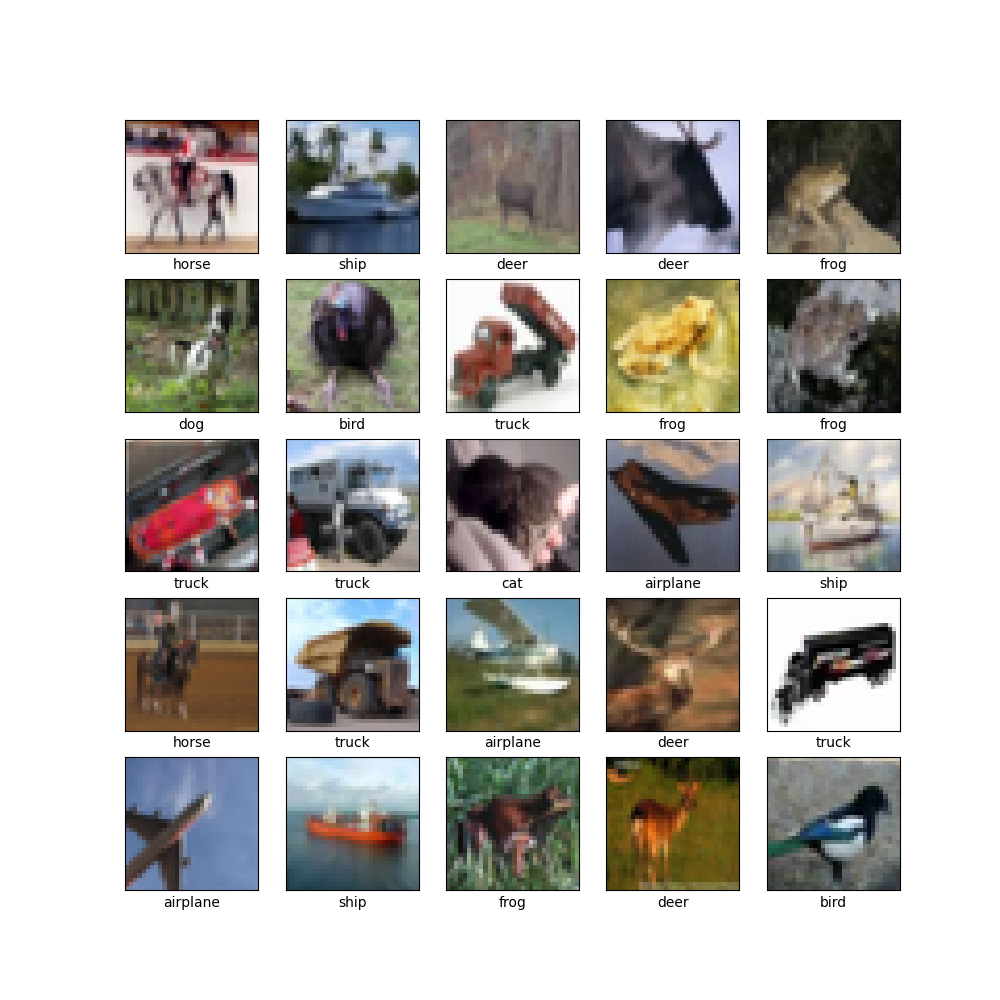
The canonical CIFAR10 dataset was used for these experiments, although experiment 3 applies a small twist to this 10 class dataset. The dataset is sourced from TensorFlow Datasets (thanks TFDS).
Experiment Design
Experiment 1
Trains two models with different architectures but similar ‘depth’
- The models are a convolutional 2D model and a densely connected neural network model
- ‘Depth’ is the number of repeated units in each model, for example a set of [a conv2d layer, and a pooling layer] are a single unit in the conv2d model. This unit is repeated N times, set at N=3 repeated units for both models in this experiment.
- Similar ‘depths’ do not necessarily yield equal trainable parameters, reference the model summaries (also below) for models Conv2D (sequential) and Dense (sequential_1). The Dense NN has an order of magnitude greater parameter count.
- NOTE: The Conv2D model includes an additional Dense layer between the last unit (conv2d, pooling) and the logits. As a result, each Dense model appends an additional Dense layer to keep this model structure constant between these model types. In other words, a Dense model with 3 layers will actually have 4 Dense layers.
Model: "sequential"
_________________________________________________________________
 Layer (type)                Output Shape              Param #
=================================================================
 conv2d (Conv2D)             (None, 30, 30, 32)        896

 max_pooling2d (MaxPooling2D  (None, 15, 15, 32)       0
 )

 conv2d_1 (Conv2D)           (None, 13, 13, 32)        9248

 max_pooling2d_1 (MaxPooling  (None, 6, 6, 32)         0
 2D)

 conv2d_2 (Conv2D)           (None, 4, 4, 32)          9248

 max_pooling2d_2 (MaxPooling  (None, 2, 2, 32)         0
 2D)

 flatten (Flatten)           (None, 128)               0

 dense (Dense)               (None, 64)                8256

 dense_1 (Dense)             (None, 10)                650

=================================================================
Total params: 28,298
Trainable params: 28,298
Non-trainable params: 0
_________________________________________________________________
 Layer (type)                Output Shape              Param #
=================================================================
 flatten_1 (Flatten)         (None, 3072)              0

 dense_2 (Dense)             (None, 64)                196672

 dense_3 (Dense)             (None, 64)                4160

 dense_4 (Dense)             (None, 64)                4160

 dense_5 (Dense)             (None, 64)                4160

 dense_6 (Dense)             (None, 10)                650

=================================================================
Total params: 209,802
Trainable params: 209,802
Non-trainable params: 0
Experiment 2
Uses two models with the same unit architecture, but different depths. In this experiment the Conv2D model is no longer used, instead two Dense NN are created with depths 3, and 6 (but actually 4 and 7, see note from experiment 1).
Of these models, the 6 (i.e., 7) depth Dense NN has 222,282 trainable parameters, or an approximate 6% increase in the number of trainable parameters over, the 3 (i.e., 4) depth Dense NN.
_________________________________________________________________
 Layer (type)                Output Shape              Param #
=================================================================
 flatten_2 (Flatten)         (None, 3072)              0

 dense_7 (Dense)             (None, 64)                196672

 dense_8 (Dense)             (None, 64)                4160

 dense_9 (Dense)             (None, 64)                4160

 dense_10 (Dense)            (None, 64)                4160

 dense_11 (Dense)            (None, 64)                4160

 dense_12 (Dense)            (None, 64)                4160

 dense_13 (Dense)            (None, 64)                4160

 dense_14 (Dense)            (None, 10)                650

=================================================================
Total params: 222,282
Trainable params: 222,282
Non-trainable params: 0
Experiment 3
Holds the model architectures constant, and trains two Dense NN models of equal depth and (approximately) the same number of trainable parameters. Instead the training and validation datasets are modified as this experiment explores the effect that the number of classes in the dataset has on MIA results.
These models have approximately the same number of trainable parameters, since the count(logits) must agree with the number of classes in the dataset, thus the 4 class, 3 Layer Dense NN has slightly lower count of trainable parameters (209,412) compared to the 10 class, 3 layer Dense NN (209,802), but this difference is negligible.
_________________________________________________________________
 Layer (type)                Output Shape              Param #
=================================================================
 flatten_3 (Flatten)         (None, 3072)              0

 dense_15 (Dense)            (None, 64)                196672

 dense_16 (Dense)            (None, 64)                4160

 dense_17 (Dense)            (None, 64)                4160

 dense_18 (Dense)            (None, 64)                4160

 dense_19 (Dense)            (None, 4)                 260

=================================================================
Total params: 209,412
Trainable params: 209,412
Non-trainable params: 0
_________________________________________________________________
Expectations & Results
Before I ran the experiments I expected:
- The model using repeated convolutional nn units should have a higher capacity of memorization
- I also expected this model to perform better at the classification task than the dense NN
- These are both consequences of the Conv2D model learning it’s filters parameters through the SGD process, these filters are better equipped to recognize features (i.e. memorize features) from our training dataset sooner in training
- More parameters should make the model overfit faster, and have a higher capacity of memorization
- A model’s ‘capacity’ is a measure of the number of trainable parameters it has, intuitively this also means its memorization capacity is greater - it can simply encode more information than smaller models
- More classes in the datasets should mean the model’s MIA attacker advantage is higher (higher MIA results)
- In the closed model attack, having more classes in the output space means there is more signal for an attacker to use in the MIA
Experiment 1
These results were as expected.
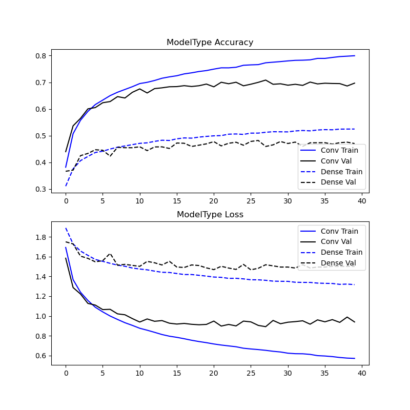
The training results demonstrate that the Conv2D layered model tends to overfit sooner, and overfit to a higher degree than the Dense NN model. This is suggested by model accuracy for the training dataset overtaking the accuracy for the validation dataset sooner (earlier in discrete epoch-timescale) and with a wider margin. The inverse is true for model loss as a matter of algebraic rearrangement.
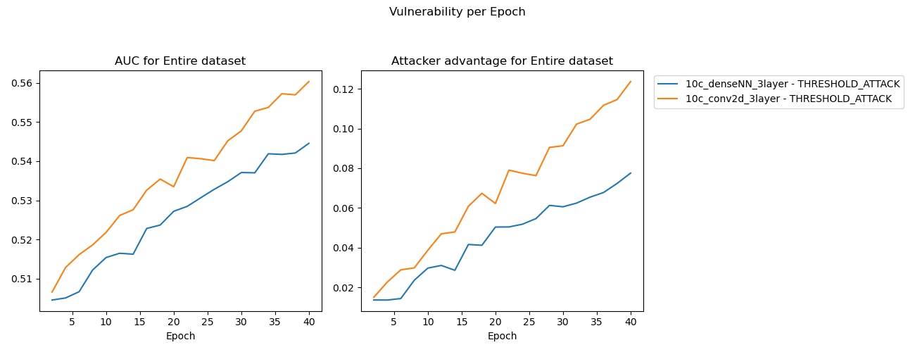
This widening margin is reinforced in the MIA threshold attack results, where again the Conv2D model tends to memorize to a higher degree than its Dense counterpart.
Hypothesis
Conv2D units encode features within its filters either from the input image matrix or the preceding layers, these filters’ values are learned during the training process. As a result, this architecture is able to encode characteristics of the input images much earlier in training than Dense connected NN are. I suspect this is the reason that despite having fewer trainable parameters (a whole order of magnitude less than the Dense NN model), the Conv2D model shows higher MIA results and faster overfitting rate.
Experiment 2
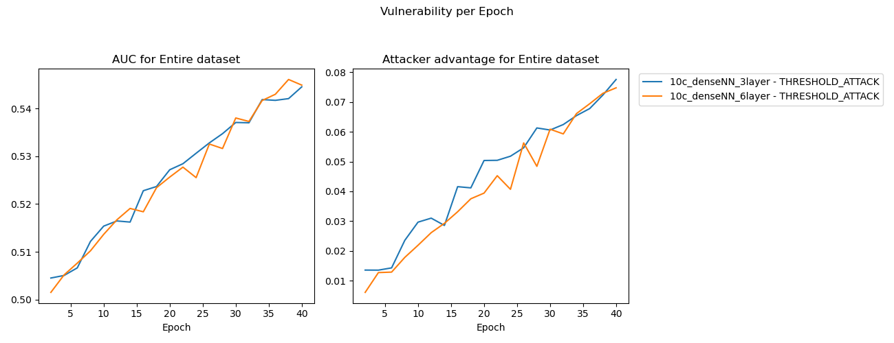
These results were inconclusive.
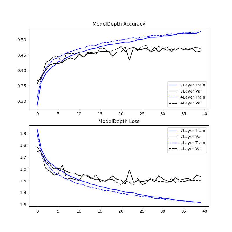
This experiment proved inconclusive, the 6% increase in trainable parameters was a marginal increase that didn’t result in a material difference in model memorization or overfitting rate. The MIA results show approximately consistent memorization between these models.
Experiment improvements: Another attempt at experiment 2 with a range of model depths (Depth = 1, 2, 4, 8, ….) holding all else as constants may yield a better basis for comparison between the results for a range of model depths.
Experiment 3
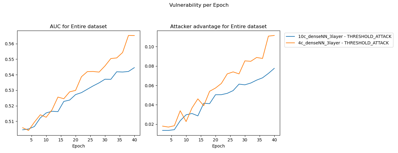
These results did not align with my expectations.
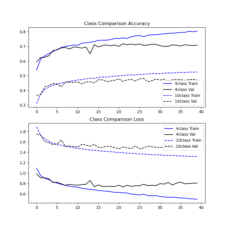
The 10 class setup begins with lower accuracy in the training results plot, which represents the fact that an untrained model guessing blindly has a lower probability of getting the right answer for a 10 class dataset (probability of 10% that a blind guess is correct) than the 4 class variant (which has a 25% of a blind guess being correct).
After training, the 4 class variant demonstrated higher MIA results and a widening margin between training and validation dataset prediction accuracies after the epoch when the model started overfitting.
Hypothesis
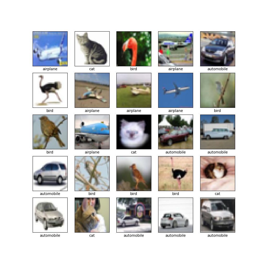
Converting the CIFAR10 to be a 4 class dataset took a naive approach: select only samples from training and validation datasets where the label is one of the first four classes. The CIFAR10 dataset is evenly distributed across its labels, this means that the 4 class dataset has (2/5) the number of samples as the 10 class.
Holding the model constant between the 10 and 4 class datasets means that there is significantly less data in each of the training and validation datasets for the 4 class dataset. It is possible that the effect of having significantly less data to work with made the 4class model overfit more and thus memorize the training samples to a higher degree than the 10class model.
Reza Shokri, Marco Stronati, Congzheng Song, & Vitaly Shmatikov. (2017). Membership Inference Attacks against Machine Learning Models. https://arxiv.org/pdf/1610.05820.pdf ↩︎ ↩︎ ↩︎
Ahmed Salem, Yang Zhang, Mathias Humbert, Pascal Berrang, Mario Fritz, & Michael Backes. (2018). ML-Leaks: Model and Data Independent Membership Inference Attacks and Defenses on Machine Learning Models. https://arxiv.org/pdf/1806.01246.pdf ↩︎
Liwei Song, & Prateek Mittal. (2020). Systematic Evaluation of Privacy Risks of Machine Learning Models. https://arxiv.org/pdf/2003.10595.pdf ↩︎ ↩︎ ↩︎
Nicholas Carlini, Steve Chien, Milad Nasr, Shuang Song, Andreas Terzis, & Florian Tramer. (2022). Membership Inference Attacks From First Principles. https://arxiv.org/pdf/2112.03570.pdf ↩︎
Yiyong Liu, Zhengyu Zhao, Michael Backes, & Yang Zhang. (2022). Membership Inference Attacks by Exploiting Loss Trajectory. https://arxiv.org/abs/2208.14933 ↩︎