Blog
Differential Privacy: Primer & Laplace Case Study
By D.Moreno
Tags: Differential Privacy, Privacy, Case Study
This post serves as a primer to Differential Privacy: presenting an intuitive foundation for the definition, proceeding to some math, and finally presenting a case study to demonstrate some key concepts.
📌 TL;DR
- Differential Privacy are a class of algorithms and a formal mathematical definition that, if met, provides an upper bound to the potential privacy loss for a query response (data release).
- The formulation stems from the intuition that we can reason about (and quantify) the privacy of some algorithm that shrouds in uncertainty whether or not a user’s data was in the dataset that informed the result.
| Differential Privacy is a definition |
|
| Differentially Private algorithms allow us to quantify the privacy loss |
|
| Epsilon is our measure of privacy loss |
|
The Theory: What is Differential Privacy
The foundation of Differential Privacy (DP) is the notion that an individual’s privacy is protected in a dataset if the individual’s contribution is simply excluded from the set of records, assuming data is independent.
Consider an algorithm that takes as input a database of user records, and outputs the average of all records. If this algorithm excluded from its calculation the contribution from a target user, or if the database did not include any contribution from that target user, then as long as records in the database were independent it follows that within the scope of what can be revealed by that algorithm the target’s data stays a secret. Specifically, DP concerns itself with shrouding in uncertainty a target’s participation in the dataset that produced the output that was released.
DP algorithms are a class of algorithms that are derived from this intuition, and that carry a mathematical guarantee for the upper-bound privacy loss of each query or data release. This mathematical formulation was the culmination of decades of privacy research, which demonstrated that prior privacy preserving standards were leaky: with enough time and repeated releases it is infeasible to make any lasting guarantee about privacy. 1 This insight motivated the development of a new standard which stemmed from the missing member in database intuition and was presented in the seminal work by C. Dwork et al. “Calibrating Noise to Sensitivity in Private Data Analysis”. 2 In their work they introduced the mathematics to describe a DP algorithm, as well as a generalized approach to implementation which, in its original or derivative forms, has since become recognized as the gold standard for privacy preserving data transformations.
From an adversarial point of view, DP roughly means that for a given query output we would be uncertain (quantifiably so) that the output was derived from a database that did or did not contain a target user’s data. Paying homage to the cryptographic roots of privacy research and differential privacy, this is analogous to semantic security in a cryptosystem.
Why was DP groundbreaking?
DP departed from previous attempts at generalized privacy preserving algorithms and standards notably with two characteristics:
- A quantification of the upper-bound privacy loss that might result for a data release
- Formalization of the privacy loss for repeated data releases from the same source data
The second of these observations is a result of DP being composable, this property allows data curators to set a global maximum privacy budget which is divided among the applications of the confidential data - the proof and practical interpretation on this later in this post.
Together, these new characteristics of the data processing mean that a system that adheres to the strict mathematical definition that is DP allows us to reason about and quantify the privacy risk against privacy attacks today as well as into the future. 3
The Math: Derivation of Differential Privacy
is said to satisfy epsilon Differential Privacy (εDP) 2
$$ \tag{1} Pr \Big(\mathbb{A}(D_1) \in S \Big) \leq \ e ^ \epsilon \cdotp Pr \Big(\mathbb{A}(D_2) \in S \Big) $$
$$ \tag{2} \frac {Pr\Big(\mathbb{A}(D_1) \in S \Big)} {Pr \Big(\mathbb{A}(D_2) \in S \Big)}\ \leq e ^ \epsilon $$
δ 4 :
$$ \tag{3} Pr \Big(\mathbb{A}(D_1) \in S \Big) \leq \ e ^ \epsilon \cdotp Pr \Big(\mathbb{A}(D_2) \in S \Big) + \delta $$
This error term can be roughly interpreted as the likelihood that the strict definition doesn’t hold. For brevity’s sake, I will introduce this here and leave as a teaser the fact that the error term can exist and that it exists to balance engineering practicality with the otherwise strict DP definition (besides… I need to save some content for future idea sharing posts! :wink:)
A quick proof… Quantifying Privacy Loss for Repeated Queries
In order to reason about the upper bound for repeated queries we need to prove that εDP is sequentially composable:
$$ \tag{4.1} Pr \Big(\mathbb{A_1}(D_1) \in \mathcal{R_1} \Big) \leq \ e ^ {\epsilon_1} \cdotp Pr \Big(\mathbb{A_1}(D_2) \in \mathcal{R_1} \Big) $$ $$ \tag{4.2} Pr \Big(\mathbb{A_2}(D_1) \in \mathcal{R_2} \Big) \leq \ e ^ {\epsilon_2} \cdotp Pr \Big(\mathbb{A_2}(D_2) \in \mathcal{R_2} \Big) $$
$$ \tag{4.3} \frac {Pr \Big(\mathbb{C}(D_1) = (r_1, r_2 ) \Big)} {Pr \Big(\mathbb{C}(D_2) = (r_1, r_2 ) \Big)} = \frac {Pr \Big(\mathbb{A_1}(D_1) = r_1 \Big)} {Pr \Big(\mathbb{A_1}(D_2) = r_1 \Big)} \frac {Pr \Big(\mathbb{A_2}(D_1) = r_2 \Big)} {Pr \Big(\mathbb{A_2}(D_2) = r_2 \Big)} $$
By a matter of substitution using Equation 2, we have:
$$ \tag{4.4} \frac {Pr \Big(\mathbb{C}(D_1) = (r_1, r_2 ) \Big)} {Pr \Big(\mathbb{C}(D_2) = (r_1, r_2 ) \Big)} \leq e ^ {\epsilon_1} e ^ {\epsilon_2} $$
$$ \tag{4.4} \frac {Pr \Big(\mathbb{C}(D_1) = (r_1, r_2 ) \Big)} {Pr \Big(\mathbb{C}(D_2) = (r_1, r_2 ) \Big)} \leq e ^ {\epsilon_1 + \epsilon_2} $$
This can be generalized for any algorithm that is the composite of N independent differentially private algorithms:
$$ \tag{4.5} \frac {Pr \Big(\mathbb{C}(D_1) = (r_1, r_2, … r_n) ) \Big)} {Pr \Big(\mathbb{C}(D_2) = (r_1, r_2, … r_n) \Big)} \leq e ^ {\epsilon_1 + \epsilon_2 + … + \epsilon_n} $$
The sum of all privacy losses is the global privacy loss, which can be divided between the N algorithms as needed. The composability of DP tells us that theoretically we can assert that at most privacy erodes linearly with respect to n-epsilons, though in practice it is sublinear.
And a bit more math… Poking at ε
$$ \tag{2} \Bigg( \frac {Pr\Big(\mathbb{A}(D_1) \in S \Big)} {Pr \Big(\mathbb{A}(D_2) \in S \Big)} \leq { e ^ \epsilon } \Bigg) {\Bigg\vert _{\epsilon \rightarrow 0}} $$
$$ \tag{2.1} \frac {Pr\Big(\mathbb{A}(D_1) \in S \Big)} {Pr \Big(\mathbb{A}(D_2) \in S \Big)} \leq 1 $$
In Practice
DP’s definition is really a conceptual property that describes a data transformation. There are a few potential transformations that satisfy this property, some popular mechanisms are additive noise mechanisms which sample noise from a distribution and inject that noise into the query response. Some popular additive noise mechanisms are:
Laplace Mechanism
This mechanism is the canonical DP mechanism that satisfies ε-DP (Equation 01), and is otherwise known as ‘pure differential privacy’. This mechanism samples noise from a zero-centered Laplace distribution and injects this noise into the data release. 2
Gaussian Mechanism
The Gaussian mechanism is very similar to the Laplace mechanism, except it uses a zero-centered, variance bound Guassian distribution and does not satisfy ε-DP, instead it satisfies (ε, δ) Differential Privacy (Equation 03). In addition to restrictions on the Noise-Distribution’s variance, this additive noise mechanism only holds true to (ε, δ) DP when ϵ < 1.
:hammer: Implementation tips
Differential Privacy is a powerful tool, while wielding it watch for:
- Dimensions in the source data that are correlated: this leads to leaky privacy guarantees
- Extreme outliers in the data: users in the long tails of data are more identifiable, require more noise to mask. Consider binning data into ranges to address this. This is also the subject of the case study
DP with Privacy Budget Accounting
Composition has been demonstrated for εDP algorithms, which allows us to define a global limit on the maximum privacy loss that we will allow for a given dataset. When this global privacy loss is set, multiple queries are each assigned some portion of the whole budget. In other words, repeated queries deplete the global privacy budget.
Referring back to Equation 02 - note that for lower ε values we expect more uncertainty in which of the datasets the algorithm’s output came from D1 or D2. As a generalization we have:
Lower ε value:
- Higher the noise we expect in the query response
- Lower accuracy in the query response as a result of the noise
- Better privacy story, but at the expense of the data utility
:wrench: ε Setting Tips
Fixing the global privacy budget means that care is needed when accounting for where to allocate higher accuracy queries, or where a sacrifice on accuracy may be made to stay within the budget.
In addition to careful accounting, cached answers can extend the budget. During the fulfillment of the query-response protocol: cache answers to queries, and retrieve cached answers when the same query is issued multiple times to the database. This type of response-replay won’t deplete the privacy budget, and ensures no additional information is learned about the data’s subjects for repeated queries.
Case Study
The following case study is hosted on GitHub, which includes a Creative Commons licensed dataset (thanks Kaggle!). In this case study we will be exploring the implementation of OpenMined PyDP which is a python wrapper that makes use of Google’s open source C++ Differential Privacy library. This Python library uses the Laplace mechanism of additive noise to satisfy εDP.
Objective: In this case study we will see the effect that:
- Different ε values have on the differential privacy noise
- Long tail skew in the source data have on differential privacy noise
The Data
For the fulfillment of this case study the data will first need to be:
- Sanitized (e.g. correct string entries in numeric columns, etc)
- Columns dropped (the data cube diced)
In addition to this clean up, we can drop all but the last month’s data for simplicity’s sake (data cube sliced). For the remainder of the case study we will be using the ‘Annual_Income‘ dimension only.

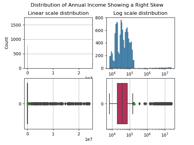
Annual Income plotted in linear and log scale
This is a terrific dimension to explore: it exhibits a rich (pun intended :moneybag:), long tailed right skew. Note that the tail is so long that it is impractical to plot annual income in linear scale (left), in log-scale we get a greater sense of where most users are and where only a few, very wealthy users are.
The Private Queries
The Git Python project includes methods for private queries:
- Repeated_average
- Repeated_sum
- Repated_max
Which take as input:
- iterations (integer) number of times the private query will be repeated
- privacy_budget (float) epsilon value, does not change between iterations
- list (array) dataframe dimension to list, that is used as source data for the private query
These methods do not use any privacy loss budget accounting, as a result over N-Iterations we expect a nice Laplace distribution in the observed query responses that should center on the true value.
Noise & ε
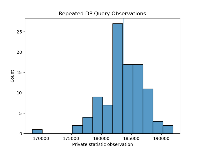
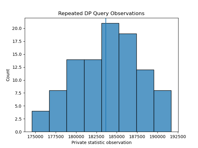
Running the repeated average method over 100 iterations, with ε = [1,100] returns the following histograms of observed query respones:

Repeated Private Average Queries, 100 iterations with Epsilon = 100

Repeated Private Average Queries, 100 iterations with Epsilon = 1
As expected, a higher ε value yields query responses with lower noise injected - demonstrated by a distribution with a tighter spread, both distributions are centered on the true value which is represented by a vertical line.
Noise & Long-tailed data
We can imagine that blending in at a crowded event is much easier than trying to blend in in an otherwise empty room; so too there is a certain degree of privacy protection among a concentrated band of data rather than in a long tail. In other words, being a member of the 107 annual income club makes it difficult to apply enough noise to mask your contribution in the annual income dataset when running a private average query.
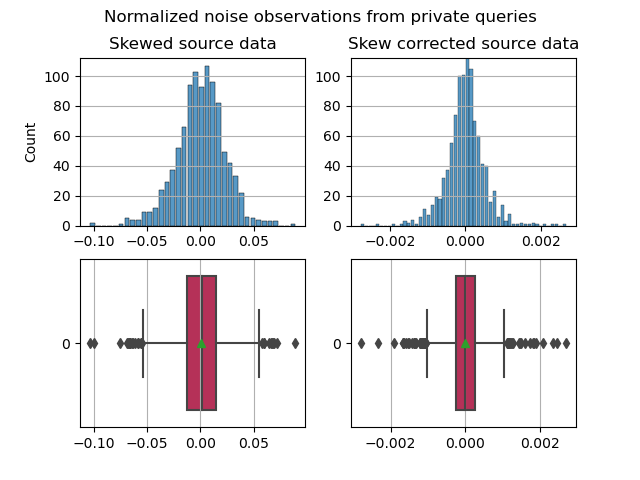
Running repeated private queries with iterations = 1000 and ε = 0.85 for the raw dataset (right skew, without any skew correction) and again for a skew-corrected dataset (still right skew, but cutting off anyone that isn’t below the 95% percentile).
For skew correction, we want to keep the count of unique users (in the dataset, count of rows) the same between datasets to make an apple to apple comparison. To address this, the skew-correction method takes any entry above 95 percentile, and replaces their contribution to annual income to be something within the sub-95 percentile band (using a random number generator within a bound).

Normalized noise observations for repeated private queries, 1000 iterations, epsilon = 0.85
These histograms are normalized to their respective distributions’ average salary. Eliminating the long tail results in over a degree of magnitude change for the normalized noise distributions. :eyes:
-
Irit Dinur and Kobbi Nissim, Revealing information while preserving privacy ↩︎
-
Cynthia Dwork, Frank McSherry, Kobbi Nissim, and Adam Smith, Calibrating noise to sensitivity in private data analysis ↩︎ ↩︎ ↩︎
-
Kobbi Nissim , Thomas Steinke , Alexandra Wood, Micah Altman, Aaron Bembenek, Mark Bun, Marco Gaboardi, David R. O’Brien, and Salil Vadhan, Differential Privacy: A Primer for a Non-technical Audience ↩︎
-
Cynthia Dwork, Krishnaram Kenthapadi, Frank McSherry, Ilya Mironov, and Moni Naor, Our data, Ourselves: Privacy via Distributions Noise Generation ↩︎